Classification

Welcome to the dataset training module!

By this point in the training, we’ve looked at much satellite imagery, often full of green vegetation, but how can we figure out exactly how much land cover is in a certain region? Classification algorithms are the answer!

In this module, we'll dive into the exciting world of classification and learn how to automate it using machine learning techniques. By importing an image and collecting training points, we can train a classifier that will help us identify different land cover types. And the best part? We can apply this classifier to the entire image and create a beautiful map that showcases the diversity of the landscape.

“If you train robots like dogs, they learn faster.”

— Kristin Houser

Advanced classification (training datasets)

Classification in Google Earth Engine (GEE) refers to the process of assigning land cover or land use categories to different geographical areas. The goal of classification is to group together pixels that have similar spectral properties or attributes into meaningful categories.

This is useful for a variety of applications, including land cover mapping, change detection, and habitat analysis. It can also be used to create thematic maps that show the distribution of different land cover classes across a region, which can be helpful for natural resource management and conservation planning. Classification is done by using Machine Learning techniques.

Background

Supervised classification uses a training dataset with known labels and representing the spectral characteristics of each land cover class of interest to “supervise” the classification. The overall approach of a supervised classification in Earth Engine is summarized as follows:

Get a scene.
Collect training data.
Select and train a classifier using the training data.
Classify the image using the selected classifier (a super simple point and click method!)

Exercise

We will use the following code to create a training dataset which will be used to autonomously classify the land around Rio de Janeiro, Brazil.

// create an Earth engine point object over rio
var pt = ee.Geometry.Point([-43.173732,-22.903846])

// Filter the landsat 8 collection and select the least cloudy image
var landsat = ee.ImageCollection('LANDSAT/LC08/C02/T1_L2')
  .filterBounds(pt)
  .filterDate('2019-01-01','2020-01-01')
  .sort('CLOUD_COVER')
  .first()

//center the map on that image
Map.centerObject(landsat,8)

//Add Landsat image to the map
var visParams = {
  bands: ['SR_B4','SR_B3','SR_B2'],
  min: 7000,
  max: 12000
};

Map.addLayer(landsat, visParams, 'Landsat 8 image');

Using the Geometry Tools, we will create points on the Landsat image that represent land cover classes of interest to use as our training data. We’ll need to do two things: (1) identify where each land cover occurs on the ground, and (2) label the points with the proper class number. For this exercise, we will use the classes and codes shown in the following table

In the Geometry Tools, click on the marker option. This will create a point geometry which will show up as an import named “geometry”. Click on the gear icon to configure this import.

We will start by collecting forest points, so name the import forest. Import it as a FeatureCollection, and then click + Property. Name the new property “class” and give it a value of 0. We can also choose a color to represent this class. For a forest class, it is natural to choose a green color. In the future, you can simply choose the color, but for this example enter the specific hexadecimal color code #589400.

Now, in the Geometry Imports, we will see that the import has been renamed forest. Click on it to activate the drawing mode in order to start collecting forest points.

Now, start collecting points over forested areas. Zoom in and out as needed. You can use the satellite basemap to assist you, but the basis of your collection should be the Landsat image. Remember that the more points you collect, the more the classifier will learn from the information you provide. For now, let’s set a goal to collect 25 points per class. Click Exit next to Point drawing when finished.

Repeat the same process for the other classes by creating new layers. Don’t forget to import using the FeatureCollection option as mentioned above. For the developed class, collect points over urban areas. For the water class, collect points over the ocean and other water features. For the herbaceous class, collect points over agricultural fields. Remember to set the “class” property for each class to its corresponding code from the table and click Exit once you finalize collecting points for each class as mentioned above. We will be using the following hexadecimal colors for the other classes: #FF0000 for developed, #1A11FF for water, and #D0741E for herbaceous.

Your training data may look something like this:

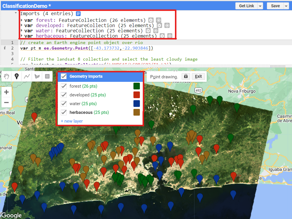
You should now have four FeatureCollection imports named forest, developed, water, and herbaceous.

The next step is to combine all the training feature collections into one. Copy and paste the code below to combine them into one FeatureCollection called trainingFeatures. Here, we use the flatten method to avoid having a collection of feature collections—we want individual features within our FeatureCollection.

// training begins
var trainingFeatures = ee.FeatureCollection([
  forest, developed, water, herbaceous
]).flatten();

Now that we have our training points, copy and paste the code below to extract the band information for each class at each point location. First, we define the prediction bands to extract different spectral and thermal information from different bands for each class. Then, we use the sampleRegions method to sample the information from the Landsat image at each point location. This method requires information about the FeatureCollection (our reference points), the property to extract (“class”), and the pixel scale (in meters).

// Define prediction bands
var predictionBands = ['SR_B1','SR_B2','SR_B3','SR_B4','SR_B5','SR_B6','SR_B7','ST_B10'
];

//Sample training points
var classifierTraining = landsat.select(predictionBands)
  .sampleRegions({
      collection: trainingFeatures,
      properties: ['class'],
      scale: 30
  });

Now it is time to choose a classification method. These are algorithms that use your training data to automatically classify all of the land in the desired area (machine learning!). One of the most common algorithms is the Classification and Regression Tree (CART) classifier. Use the code below to implement the CART classifier.

// Train a CART classifier
var classifier = ee.Classifier.smileCart().train({
  features: classifierTraining,
  classProperty: 'class',
  inputProperties: predictionBands
})

Now that you’ve trained the classifier, simply use the code below to classify the Landsat image and add it to the Map.

// Classify the landsat image
var classified = landsat.select(predictionBands).classify(classifier);

// Define classification image visualization parameters
var classificationVis = {
  min: 0,
  max: 3,
  palette: ['589400','ff0000','1a11ff','d0741e']
};

// Add the classified image to the map
Map.addLayer(classified, classificationVis, 'CART classified')

Phew! We just learned a lot! Slow down, look through the code line by line, and think about what each chunk does. In summary:

We imported a LANDSAT image then filtered it by date and location. Then we added this image as a layer to the map
We created point geometries to use as training points for our classification algorithm (using a simple point and click technique!)
We added these training points to a variable called trainingFeatures, then added bands to our variable predicitonBands for our classifier to use.
We used these variables as inputs to train our CART classifier
Our classifier is now trained, so we used it to classify the rest of our image automatically and display the results!

Results

Inspect the result: Activate the Landsat composite layer and the satellite basemap to overlay with the classified images. Change the layers’ transparency to inspect some areas. What do you notice? The result might not look very satisfactory in some areas (e.g., confusion between developed and herbaceous classes). Why do you think this is happening?

Here are some ways we can improve our classification code:

Collect more training data We can try incorporating more points to have a more representative sample of the classes.

Try other classifiers If a classifier’s results are unsatisfying, we can try some of the other classifiers in Earth Engine to see if the result is better or different.
Expand the collection location It is good practice to collect points across the entire image and not just focus on one location. Also, look for pixels of the same class that show variability (e.g., for the developed class, building rooftops look different than house rooftops; for the herbaceous class, crop fields show distinctive seasonality/phenology).
Add more predictors We can try adding spectral indices to the input variables; this way, we are feeding the classifier new, unique information about each class. For example, there is a good chance that a vegetation index specialized for detecting vegetation health (e.g., NDVI) would improve the developed versus herbaceous classification.

Recap

This training was jam packed.

Here’s what we learned in this training:

Classification algorithms are useful for determining land cover and resource management in a region - and can be automated through machine learning!
We simply import an image, collect training points, train the classifier, then apply the trained classifier to the rest of our image

New code elements:

There are a plethora of new code elements here. This is a great code to copy and paste, then alter as you see fit for your application. Add more classes or take some away! Change the colors if you’d like. Be creative in classifying new, meaningful things for your application.